Due to its popularity and ease of use, Microsoft Excel has become the default tool when it comes to quickly prototyping an idea, model, or even a simple trading strategy. Although there are plenty of sophisticated backtesting websites or libraries for every programming language imaginable, it is still a good idea to know how to create a backtest manually in order to make sure we understand what is going on.

In this article, I’ll go through a step-by-step example showing how to backtest a simple strategy consisting of two moving averages that cross each other and create buy and sell signals.

In order to create a strategy using Microsoft Excel, we first have to get historical data and calculate the indicators. The next step consists in using said indicators to create the trading rules that will generate the buy and sell signals. Finally, the last step consists in calculating the return of the strategy and its benchmark, in addition to other metrics that are commonly used in the industry.

Before getting started with this tutorial, it is worth mentioning that you’ll probably be able to backtest much more efficiently using BacktestXL. This backtesting engine works natively in Microsoft Excel and also fetches historical stock prices and alternative datasets. It also calculates technical indicators and has pattern recognition functions. Disclaimer: we’re the developers, but it really is the software we use for our personal research!

You can also follow along with the video at the end of the article, which exactly replicates the article.

Getting Historical Data for Microsoft Excel

To get started, we can go to Yahoo Finance and download historical data. Although limited to just a few days, this source allows downloading intraday data. You just have to go to finance.yahoo.com, select a stock, click on the “Historical Data” tab, select the desired time period and frequency and click on “Download.”

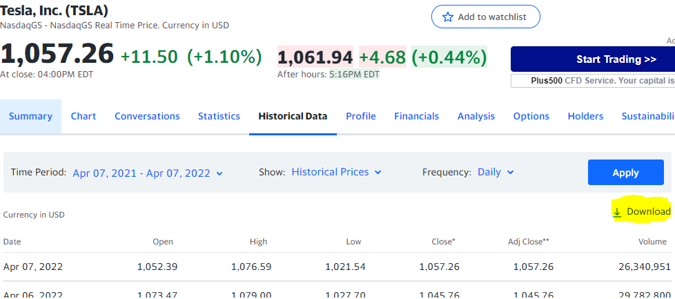
Having said that, if you want to replicate the exact results of this article, download the raw data from this link: Download Initial Worksheet.

Calculate Trading Indicators in Excel

In this article, we will use two moving averages with different lengths. The first one, which we will call “Fast SMA”, will cover the last 8 prices, whereas the “Slow SMA” will be the average of the last 16 periods.

Since we will only be using the closing prices, delete the columns for the Open, High, Low, Volume, Dividends, and Stock Splits. You will have the dates in Column A and the closing price in Column B.

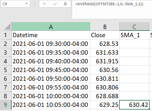
We can use the “=average()” function in order to calculate both moving averages (MAs). But to allow for easily changing the number of periods covered by each MA, we will use the offset function to parameterize the number of rows used for the calculation.

Let’s break this down step by step:

• Offset function:

1. We instruct the function to start in cell B9 and move one cell up (-1). We move one cell up to avoid lookahead bias (using data that is not available to us at the moment of creating a signal). From there, we have to specify the height and width of the range.
2. The height will be “-SMA”, where SMA is a named cell with the value 8.
3. We also specify the width of the range to be 1, since we just want to select column B

• Average

1. The previous step created a range of 8 closing price values. Now, all that’s left to do is to wrap that function inside and AVERAGE() function, while will return the average of the 8 cells.

Repeat the same step in Column D for the second SMA (slow). Refer to the video at the end if you are having issues. Don’t forget to apply these formulas to the entire time series (fill the columns).

Create Trading Rules or Signals in Excel

The following step consists in establishing the rules that we will follow to buy and sell the asset. We will hold the stock when the fast-moving average is greater than the slow-moving average. Conversely, we won’t hold the asset whenever the fast-moving average is smaller than the slow-moving average.

In column E, we will do that calculation. For example, the formula in cell E17 would be:

=C17>D17

This will return TRUE or FALSE, telling us at any given time if we are holding the asset. In other words, whenever we switch from FALSE to TRUE, we are buying the underlying stock, and when we switch from TRUE to FALSE, we can conclude that we sold it. Fill the remaining cells from column E with the same formula.

Calculating the Performance of a Trading Strategy in Excel

Returns of the Buy and Hold Benchmark

We now have to calculate the performance of our trading strategy. We will also calculate the returns of the Buy & Hold Strategy to use it as a benchmark. The B&H is none other than buying in the first period and selling in the last one. In other words, it is the asset’s return over the entire time horizon.

In order to calculate the returns, we will use logarithmic returns instead of the usual arithmetic ones. This is because the sum of the logarithmic returns of every period is the same as the returns over the entire period, which is very convenient for computational reasons. Calculating cumulative arithmetic returns would be computationally expensive with larger datasets and is thus considered a bad practice. Also, once you understand logarithmic returns, you will conclude that they are better suited for the current task at hand.

To calculate the logarithmic return: in cell B3, use the following formula:

=LN(B3/B2)
/////////////////////
This is the logarithm of todays price divided by yesterdays.

Now you can apply this formula to the remaining cells in the series.

If you SUM the entire range of logarithmic returns, you will get the returns of holding the asset. In other words, that sum is the same as taking the last price and dividing it by the first price. That is the return of the B&H Strategy.

Returns of the strategy

Now, let’s calculate the returns of our strategy, which is none other than the sum of the daily returns where we had a position in the stock (cells in column E are TRUE). For the remaining days, our strategy did not have any return since we were holding cash instead of the asset. For cell G3, the formula is the following:

=IF(E3=TRUE,F3,0)
/////////////////////
The IF function takes the following three parameters:
1. The condition to be evaluated
2. The value returned if the condition is met
3. The value returned if the condition is false 

Now, if we calculate a SUM over the entire column, we will get the return of our strategy. Herein lies the suitability of the logarithmic returns.

Exposure Time

Exposure time measures the percentage of days we are exposed to the volatility of the asset. In other words, it is the ratio of the number of periods where we held a position (column G is TRUE) over the total number of periods of the backtests.

In any given cell, use the following formula to calculate exposure time:

=COUNTIF(E2:E4680,TRUE)/COUNTA(E2:E4680)
/////////////////////
-The numerator (COUNTIF) counts the number of cells where the value is TRUE (i.e: holding a position
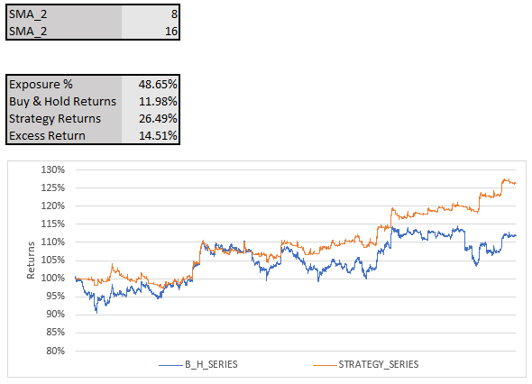
-The denominator (COUNTA) counts the total number of cells selected.

I also added two columns, one for the cumulative return of the B&H and another one for our strategy. Finally, I created a time series chart to visualize the evolution of both. I won’t be covering this final step since the article is already quite long, but you can find it in the final file with the strategy.

The final result of our strategy looks as follows:

A Warning on Backtesting a Strategy

If you followed along with this tutorial using the file provided, you’ll notice that the returns of the strategy are greater than the ones we would have obtained by just buying.

This is very much on purpose since I tweaked the parameters of both the fast and slow MAs to yield good performance. Most probable than not, we are guilty of overfitting. In other words, I tweaked the parameters in order to obtain good results on past data, but this won’t be indicative of good future performance.

If you want to tweak a strategy without increasing the risk of overfitting, consider splitting the dataset into two periods. Design the strategy with the first period and only use the second period to test if the results are similar. If you go back and forth between both periods, you’ll be overfitting again.

Additionally, trading with a strategy instead of just holding the asset has many consequences. The most relevant are the following:

• Less Volatility (exposure time): by not always having a position on the asset, you are reducing the strategy’s volatility since holding cash has zero volatility (in nominal terms). This can lead to missing a price increase, but also to avoid being exposed to the asset during a significant downturn.
• Trading Fees: some brokers charge a fee for every transaction, which should be accounted for when backtesting a strategy. In this article, we assume no fees are charged.
• Slippage: it is the difference between the expected price and the real average purchase price of the purchase. This is due to the bid-ask spread. Slippage increases when an asset features higher volatility and low liquidity. Slippage is also greater when market orders are employed since they buy at the ask and sell at the bid.

Video Tutorial of the Article