In this article, we will continue building a backtesting engine from scratch. We will add many features and make many changes, so make sure to read Part 1 of this series before reading this article!

As a quick recap, in Part 1 of this series, we’ve laid out the basics of any backtesting framework:

• Designed the structure of our framework: implemented Engine, Order, Trade, and Strategy classes
• Basic methods: run(), add_data(), buy(), sell(), add_strategy(), on_bar()
• Basic output: once the backtest is complete, the engine will calculate the strategy’s total return.
• Sanity check: we’ve compared our results with Backtesting.py

Although we can already do a whole lot of backtesting with what we’ve implemented, we surely would like to expand the framework’s capabilities! In this article, I’ll cover the following topics:

• Limit orders: implementing orders with limited prices requires refactoring some classes and methods
• Add a Benchmark: We will add a Buy & Hold strategy for the same asset for comparison purposes.
• Output Statistics: annualized returns, volatility, Sharpe Ratio, and Maximum Drawdown for both the strategy and the benchmark. Exposure of our strategy to the asset as a percentage of total assets under management.
• Plotting features: every backtesting engine out there has plotting capabilities, and our framework will not be the exception!

For organizational purposes, I’ll break down this tutorial into different sections. I’ll start by adding the limit orders.

Implementing Limit Orders

This feature impacts quite a few parts of our backtesting engine. Let’s try not to break everything!

1) Add buy_limit and sell_limit methods to our Strategy class

These methods are similar to the market buy and sell methods we created in Part 1 but with a few obvious extra parameters.

def buy_limit(self,ticker,limit_price, size=1):
    self.orders.append(
        Order(
            ticker = ticker,
            side = 'buy',
            size = size,
            limit_price=limit_price,
            order_type='limit',
            idx = self.current_idx
        ))

def sell_limit(self,ticker,limit_price, size=1):
    self.orders.append(
        Order(
            ticker = ticker,
            side = 'sell',
            size = -size,
            limit_price=limit_price,
            order_type='limit',
            idx = self.current_idx
        ))

2) Add limit_price and order_type attributes to the Order Class

class Order():
    def __init__(self, ticker, size, side, idx, limit_price=None, order_type='market'):
        ...
        self.type = order_type
        self.limit_price = limit_price

3) Update the _fill_orders() method

This section is definitely the most complex of the implementation, so make sure to read it line by line. I added a few comments to guide you through the logic.

We’ll throw in a few print statements to simplify debugging. Once we’re done testing the logic, we can remove them.

def _fill_orders(self):
    for order in self.strategy.orders:
        # FOR NOW, SET FILL PRICE TO EQUAL OPEN PRICE. THIS HOLDS TRUE FOR MARKET ORDERS
        fill_price = self.data.loc[self.current_idx]['Open']
        can_fill = False
        if order.side == 'buy' and self.cash >= self.data.loc[self.current_idx]['Open'] * order.size:
            if order.type == 'limit':
                # LIMIT BUY ORDERS ONLY GET FILLED IF THE LIMIT PRICE IS GREATER THAN OR EQUAL TO THE LOW PRICE
                if order.limit_price >= self.data.loc[self.current_idx]['Low']:
                    fill_price = order.limit_price
                    can_fill = True
                    print(self.current_idx, 'Buy Filled. ', "limit",order.limit_price," / low", self.data.loc[self.current_idx]['Low'])

                else:
                    print(self.current_idx,'Buy NOT filled. ', "limit",order.limit_price," / low", self.data.loc[self.current_idx]['Low'])
            else:        
                can_fill = True 
        elif order.side == 'sell' and self.strategy.position_size >= order.size:
            if order.type == 'limit':
                #LIMIT SELL ORDERS ONLY GET FILLED IF THE LIMIT PRICE IS LESS THAN OR EQUAL TO THE HIGH PRICE
                if order.limit_price <= self.data.loc[self.current_idx]['High']:
                    fill_price = order.limit_price
                    can_fill = True
                    print(self.current_idx,'Sell filled. ', "limit",order.limit_price," / high", self.data.loc[self.current_idx]['High'])

                else:
                    print(self.current_idx,'Sell NOT filled. ', "limit",order.limit_price," / high", self.data.loc[self.current_idx]['High'])
            else:
                can_fill = True
                
        if can_fill:
            t = Trade(
                ticker = order.ticker,
                side = order.side,
                price= fill_price,
                size = order.size,
                type = order.type,
                idx = self.current_idx)

            self.strategy.trades.append(t)
            self.cash -= t.price * t.size

    self.strategy.orders = []

By clearing the list of pending orders at the end of the method, we are assuming that limit orders are only valid for the day. This behavior tends to be the default. Implementing good till-granted (GTC) orders would require us to keep all unfilled limit orders.

4) Add a close property in the Strategy class to retrieve the latest close

This property will allow us to access the current close with a simple self.close line in the Strategy class. Although not strictly required, it is very convenient for setting the limit prices of our orders (ie, limit_price = self.close * 0.995)

Add this property to the Strategy base class

@property
def close(self):
    return self.data.loc[self.current_idx]['Close']

5) Testing the feature

Let’s use the BuyAndSellSwitch strategy we created in the previous article to review the limit orders.

In this simple scenario, we will try to buy and sell at a slightly more convenient price. In other words, our buy orders will have a limit price below the latest close, whereas our sell orders will have a limit price above it.

import yfinance as yf
class BuyAndSellSwitch(Strategy):
    def on_bar(self):
        if self.position_size == 0:
            limit_price = self.close * 0.995
            self.buy_limit('AAPL', size=100,limit_price=limit_price)
            print(self.current_idx,"buy")
        else:
            limit_price = self.close * 1.005
            self.sell_limit('AAPL', size=100,limit_price=limit_price)
            print(self.current_idx,"sell")
            
data = yf.Ticker('AAPL').history(start='2022-12-01', end='2022-12-31', interval='1d')
e = Engine()
e.add_data(data)
e.add_strategy(BuyAndSellSwitch())
e.run()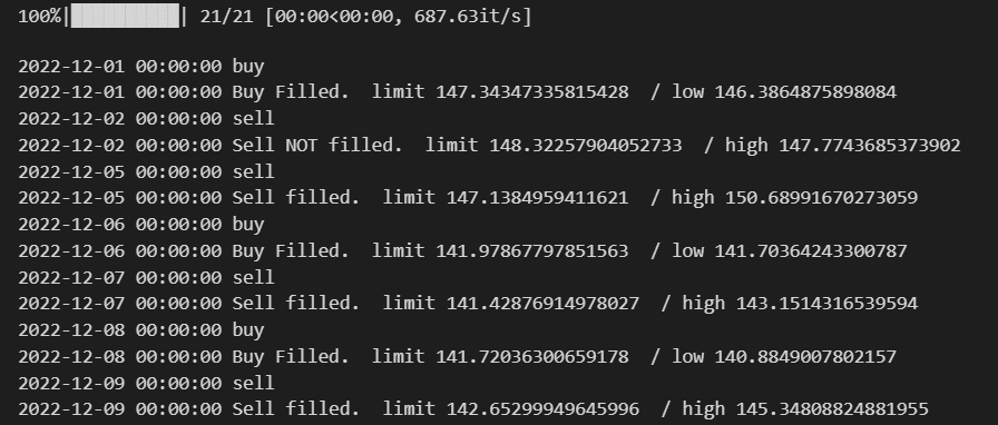   

At first sight, the code seems to be working properly. Our first sell order did not get filled because we had a limit price greater than the high. A sell order did get filled on the next bar because our limit price was lower than the day’s high. This behavior is correct!

Adding Output Metrics

We’ll want to keep track of our cash and stock holdings in each period. This will allow us to calculate the exposure of our portfolio to the market. It is also a prerequisite for calculating annualized volatility. We’ll also want to keep track of our position size.

In the __init__() method of the Engine class, create an empty dictionary for holding the cash series and another for the stock series. The sum of both values in each period equals the total assets under management.

class Engine():
    def __init__(self, initial_cash=100_000):
        ...
        self.cash_series = {}
        self.stock_series = {}

After each iteration in the run() method of the Engine class, add the cash holdings to the cash_series:

def run(self):    
    ...
    for idx in tqdm(self.data.index):
        ...
        self.cash_series[idx] = self.cash
        self.stock_series[idx] = self.strategy.position_size * self.data.loc[self.current_idx]['Close']

Now it’s time to add a few extra metrics to our engine! We’ll add those in the _get_stats method() that gets invoked at the end of the run() method.

def _get_stats(self):
    metrics = {}
    ...
    return metrics

We’ll be using the numpy library, so make sure to install it! (pip install numpy).

I’ll break down the additions to the _get_stats() method into smaller bits.

Buy & Hold Benchmark

The benchmark consists of buying as many shares as our cash allows us to in the first bar and holding them throughout the entire backtesting period.

portfolio_bh = self.initial_cash / self.data.loc[self.data.index[0]]['Open'] * self.data.Close

Exposure to the Asset [%]

We will define the exposure to the asset as a ratio of stock holdings over total assets under management at each period. Thus the average exposure of the strategy will be the average exposure of all bars.

We’ll start by creating a DataFrame containing the cash and stock holdings series and another column with the total assets under management. Finally, we have to calculate the average of the ratio.

# Create a dataframe with the cash and stock holdings at the end of each bar
portfolio = pd.DataFrame({'stock':self.stock_series, 'cash':self.cash_series})
# Add a third column with the total assets under managemet
portfolio['total_aum'] = portfolio['stock'] + portfolio['cash']
# Caclulate the total exposure to the asset as a percentage of our total holdings
metrics['exposure_pct'] = ((portfolio['stock'] / portfolio['total_aum']) * 100).mean()

Annualized Returns

# Calculate annualized returns
p = portfolio.total_aum
metrics['returns_annualized'] = ((p.iloc[-1] / p.iloc[0]) ** (1 / ((p.index[-1] - p.index[0]).days / 365)) - 1) * 100
p_bh = portfolio_bh
metrics['returns_bh_annualized'] = ((p_bh.iloc[-1] / p_bh.iloc[0]) ** (1 / ((p_bh.index[-1] - p_bh.index[0]).days / 365)) - 1) * 100

Annualized Volatility

For this calculation,

I’m assuming we’re using daily data of an asset that trades only during working days (i.e., stocks). If you’re trading cryptocurrencies, use 365 instead of 252.

self.trading_days = 252
metrics['volatility_ann'] = p.pct_change().std() * np.sqrt(self.trading_days) * 100
metrics['volatility_bh_ann'] = p_bh.pct_change().std() * np.sqrt(self.trading_days) * 100

I added a trading_days attribute to the Engine Class. Consider adding it as a parameter during the initialization of the object instead of here.

Sharpe Ratio

Now that we have the annualized returns and volatility, we can calculate the Sharpe Ratio. Keep in mind that the Sharpe Ratio also uses the risk-free rate. For simplicity, I’m assuming a risk-free rate of 0. You should define the risk_free_rate in the __init__() method instead of here.

self.risk_free_rate = 0
metrics['sharpe_ratio'] = (metrics['returns_annualized'] - self.risk_free_rate) / metrics['volatility_ann']
metrics['sharpe_ratio_bh'] = (metrics['returns_bh_annualized'] - self.risk_free_rate) / metrics['volatility_bh_ann']

Maximum Drawdown

This metric is tough to implement, so I’ll break it down into smaller bits and add plots to make it easier to understand what’s happening under the hood.

I have also not found a good online resource covering the step-by-step process. What are new articles for if not for adding new information to the internet?

We’ll be plotting quite a lot, so let’s start by importing a few libraries:

# Import matplotlib
import matplotlib.pyplot as plt
# Setting a nice style for the plots
import seaborn as sns
sns.set_style('darkgrid')
# Make plots bigger
plt.rcParams['figure.figsize'] = [20,12]

I will be using the daily prices of AAPL stock during the 2008 crisis.

data = yf.Ticker('AAPL').history(start='2007-12-01', end='2009-12-31', interval='1d')
close = data.Close
close.plot()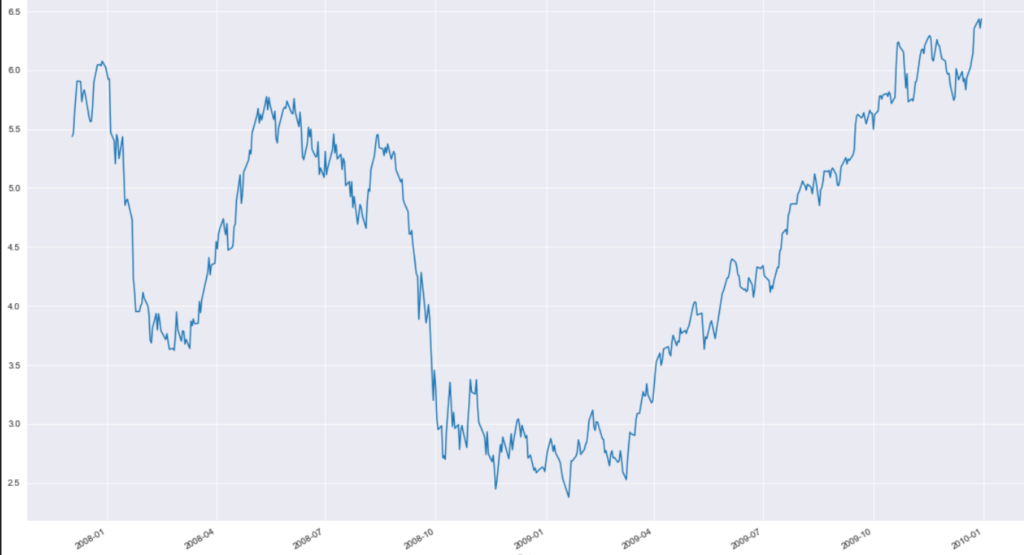

Let’s keep track of the cumulative maximum of the rolling series. Don’t worry; it will make sense later on!

roll_max = close.cummax()
roll_max.plot()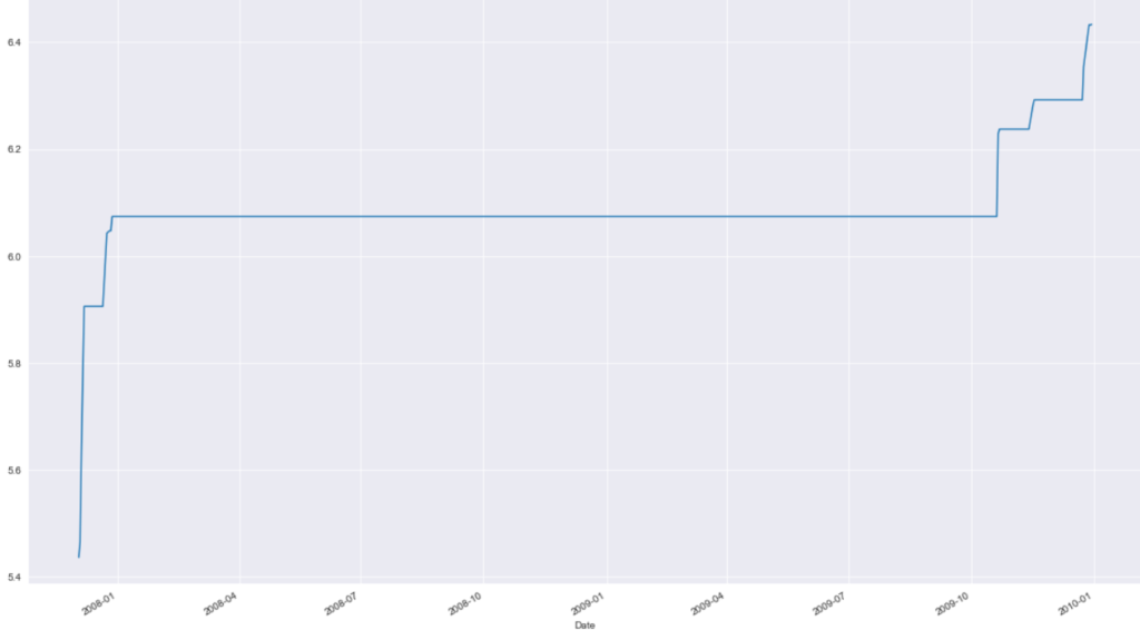

We can now calculate each day’s drawdown relative to the past maximum value.

daily_drawdown = close / roll_max - 1.0
daily_drawdown.plot()

We’re almost done! Let’s keep track of the rolling minimum drawdown:

max_daily_drawdown = daily_drawdown.cummin()
max_daily_drawdown.plot()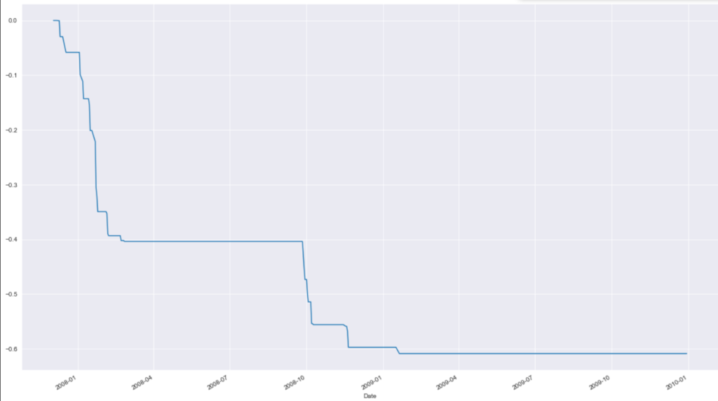

If we take the minimum value of the series, we’ll arrive at the maximum drawdown! Let’s put it all together in a single function that we can use:

def get_max_drawdown(close):
    roll_max = close.cummax()
    daily_drawdown = close / roll_max - 1.0
    max_daily_drawdown = daily_drawdown.cummin()
    return max_daily_drawdown.min() * 100

Extra data for later use

For plotting purposes, we’ll store the portfolio series.

self.portfolio = portfolio
self.portfolio_bh = portfolio_bh

Sanity Checks

Let’s implement a simple backtest to check if our metrics are reasonable! I’ll replicate a Buy & Hold strategy and compare it to the benchmark results.

import yfinance as yf
class Test1(Strategy):
    def on_bar(self):
        if self.position_size == 0:
            limit_price = self.close * 0.995
            # We'll try to buy spend all our available cash!
            self.buy_limit('AAPL', size=8.319, limit_price=limit_price)
            print(self.current_idx,"buy")
            
data = yf.Ticker('AAPL').history(start='2020-12-01', end='2022-12-31', interval='1d')
e = Engine(initial_cash=1000)
e.add_data(data)

e.add_strategy(Test1())
e.run()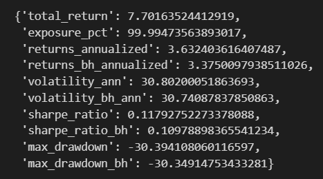

As we can see, the results don’t quite match. This is because I rounded the initial buy limit order to the third decimal. Moreover, we created the order with a limit_price, which got executed on the next open, whereas the benchmark buys in the first period with a market order at the open price.

Implementing an SMA Crossover Strategy

At last, let’s backtest something interesting! For this strategy, we will use the following indicators:

• 12-day simple moving average
• 24-day simple moving average

Whenever the 12-day moving average crosses above the 24-day moving average, we will buy. Conversely, whenever the 12-day moving average crosses below the 24-day moving average, we will sell.

It would be nice to buy as many stocks as our cash allows at any given time instead of always trading a fixed number of stocks. To do so, we would need access to the cash attribute in the Strategy class, but we are currently storing that attribute in the Engine class.

To add this feature, do the following:

• Add the following line in the Strategy’s __init__() method: self.cash = None
• At the start of the run() method, add the following line: self.strategy.cash = self.cash
• At the end of the _fill_orders() method, add the following line: self.cash = self.strategy.cash. Make sure to add it after updating the cash variable of the engine object.

Once we’ve added this feature, we can implement the strategy!

import yfinance as yf
class SMACrossover(Strategy):
    def on_bar(self):
        if self.position_size == 0:
            if self.data.loc[self.current_idx].sma_12 > self.data.loc[self.current_idx].sma_24:
                limit_price = self.close * 0.995
                # BUY AS MANY SHARES AS WE CAN!
                order_size = self.cash / limit_price
                self.buy_limit('AAPL', size=order_size, limit_price=limit_price)
        elif self.data.loc[self.current_idx].sma_12 < self.data.loc[self.current_idx].sma_24:
            limit_price = self.close * 1.005
            self.sell_limit('AAPL', size=self.position_size, limit_price=limit_price)
            
data = yf.Ticker('AAPL').history(start='2010-12-01', end='2022-12-31', interval='1d')
e = Engine(initial_cash=1000)

data['sma_12'] = data.Close.rolling(12).mean()
data['sma_24'] = data.Close.rolling(24).mean()
e.add_data(data)

e.add_strategy(SMACrossover())
stats = e.run()
print(stats)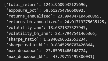

As can be seen, this simple strategy had outstanding results during the backtesting period, and for a good reason: I tweaked the parameters until they yielded good results. This practice is known as overfitting and is a very bad one! Thus, the resulting strategy is equally terrible and only meant to show how to use our newly coded backtesting engine.

Our backtest had almost identical returns compared to the buy and held benchmark but a much higher Sharpe Ratio. The lower exposure percentage explains this, which results in a much lower annualized volatility.

Add Plotting Features

Let’s end this article on a high note! What’s nicer than looking at a price chart that goes up and to the right? Let’s create the feature that will allow us to visualize that chart!

It is extremely simple, but it serves as a good starting point. Make sure to add it as a method of the Engine class.

def plot(self):
    plt.plot(self.portfolio['total_aum'],label='Strategy')
    plt.plot(self.portfolio_bh,label='Buy & Hold')
    plt.legend()
    plt.show()

We can now plot the results by calling the method after running the backtest!

e.plot()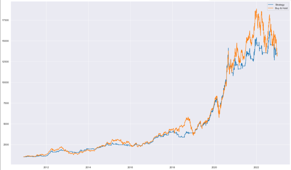

Putting Everything Together

If we put everything together, our backtesting framework should look as follows:

import seaborn as sns
import matplotlib.pyplot as plt
plt.rcParams['figure.figsize'] = [20, 12]

import pandas as pd
from tqdm import tqdm
import numpy as np

class Order():
    def __init__(self, ticker, size, side, idx, limit_price=None, order_type='market'):
        self.ticker = ticker
        self.side = side
        self.size = size
        self.type = order_type
        self.limit_price = limit_price
        self.idx = idx
        
class Trade():
    def __init__(self, ticker,side,size,price,type,idx):
        self.ticker = ticker
        self.side = side
        self.price = price
        self.size = size
        self.type = type
        self.idx = idx
    def __repr__(self):
        return f'<Trade: {self.idx} {self.ticker} {self.size}@{self.price}>'

class Strategy():
    def __init__(self):
        self.current_idx = None
        self.data = None
        self.cash = None
        self.orders = []
        self.trades = []
    
    def buy(self,ticker,size=1):
        self.orders.append(
            Order(
                ticker = ticker,
                side = 'buy',
                size = size,
                idx = self.current_idx
            ))

    def sell(self,ticker,size=1):
        self.orders.append(
            Order(
                ticker = ticker,
                side = 'sell',
                size = -size,
                idx = self.current_idx
            ))
        
    def buy_limit(self,ticker,limit_price, size=1):
        self.orders.append(
            Order(
                ticker = ticker,
                side = 'buy',
                size = size,
                limit_price=limit_price,
                order_type='limit',
                idx = self.current_idx
            ))

    def sell_limit(self,ticker,limit_price, size=1):
        self.orders.append(
            Order(
                ticker = ticker,
                side = 'sell',
                size = -size,
                limit_price=limit_price,
                order_type='limit',
                idx = self.current_idx
            ))
        
    @property
    def position_size(self):
        return sum([t.size for t in self.trades])

    @property
    def close(self):
        return self.data.loc[self.current_idx]['Close']
        
    def on_bar(self):
        """This method will be overriden by our strategies.
        """
        pass

class Engine():
    def __init__(self, initial_cash=100_000):
        self.strategy = None
        self.cash = initial_cash
        self.initial_cash = initial_cash
        self.data = None
        self.current_idx = None
        self.cash_series = {}
        self.stock_series = {}
        
    def add_data(self, data:pd.DataFrame):
        # Add OHLC data to the engine
        self.data = data
        
    def add_strategy(self, strategy):
        # Add a strategy to the engine
        self.strategy = strategy

    
    def run(self):
        # We need to preprocess a few things before running the backtest
        self.strategy.data = self.data
        self.strategy.cash = self.cash
        
        for idx in tqdm(self.data.index):

            self.current_idx = idx
            self.strategy.current_idx = self.current_idx
            # fill orders from previus period
            self._fill_orders()
            
            # Run the strategy on the current bar
            self.strategy.on_bar()
            self.cash_series[idx] = self.cash
            self.stock_series[idx] = self.strategy.position_size * self.data.loc[self.current_idx]['Close']
        return self._get_stats()
                
    def _fill_orders(self):
        for order in self.strategy.orders:
            # FOR NOW, SET FILL PRICE TO EQUAL OPEN PRICE. THIS HOLDS TRUE FOR MARKET ORDERS
            fill_price = self.data.loc[self.current_idx]['Open']
            can_fill = False
            if order.side == 'buy' and self.cash >= self.data.loc[self.current_idx]['Open'] * order.size:
                if order.type == 'limit':
                    # LIMIT BUY ORDERS ONLY GET FILLED IF THE LIMIT PRICE IS GREATER THAN OR EQUAL TO THE LOW PRICE
                    if order.limit_price >= self.data.loc[self.current_idx]['Low']:
                        fill_price = order.limit_price
                        can_fill = True
                        print(self.current_idx, 'Buy Filled. ', "limit",order.limit_price," / low", self.data.loc[self.current_idx]['Low'])

                    else:
                        print(self.current_idx,'Buy NOT filled. ', "limit",order.limit_price," / low", self.data.loc[self.current_idx]['Low'])
                else:        
                    can_fill = True 
            elif order.side == 'sell' and self.strategy.position_size >= order.size:
                if order.type == 'limit':
                    #LIMIT SELL ORDERS ONLY GET FILLED IF THE LIMIT PRICE IS LESS THAN OR EQUAL TO THE HIGH PRICE
                    if order.limit_price <= self.data.loc[self.current_idx]['High']:
                        fill_price = order.limit_price
                        can_fill = True
                        print(self.current_idx,'Sell filled. ', "limit",order.limit_price," / high", self.data.loc[self.current_idx]['High'])

                    else:
                        print(self.current_idx,'Sell NOT filled. ', "limit",order.limit_price," / high", self.data.loc[self.current_idx]['High'])
                else:
                    can_fill = True
                    
            if can_fill:
                t = Trade(
                    ticker = order.ticker,
                    side = order.side,
                    price= fill_price,
                    size = order.size,
                    type = order.type,
                    idx = self.current_idx)

                self.strategy.trades.append(t)
                self.cash -= t.price * t.size
                self.strategy.cash = self.cash
        # BY CLEARING THE LIST OF PENDING ORDERS, WE ARE ASSUMING THAT LIMIT ORDERS ARE ONLY VALID FOR THE DAY
        # THIS TENDS TO BE THE DEFAULT. IMPLEMENTING GOOD TILL GRANTED WOULD REQUIRE US TO KEEP ALL UNFILLED LIMIT ORDERS.
        self.strategy.orders = []
            

    def _get_stats(self):
        
        metrics = {}
        total_return = 100 *((self.data.loc[self.current_idx]['Close'] * self.strategy.position_size + self.cash) / self.initial_cash -1)
        metrics['total_return'] = total_return
            # Create a the Buy&Hold Benchmark
        portfolio_bh = (self.initial_cash / self.data.loc[self.data.index[0]]['Open']) * self.data.Close
        # Create a dataframe with the cash and stock holdings at the end of each bar
        portfolio = pd.DataFrame({'stock':self.stock_series, 'cash':self.cash_series})
        # Add a third column with the total assets under managemet
        portfolio['total_aum'] = portfolio['stock'] + portfolio['cash']
        # Caclulate the total exposure to the asset as a percentage of our total holdings
        metrics['exposure_pct'] = ((portfolio['stock'] / portfolio['total_aum']) * 100).mean()
        # Calculate annualized returns
        p = portfolio.total_aum
        metrics['returns_annualized'] = ((p.iloc[-1] / p.iloc[0]) ** (1 / ((p.index[-1] - p.index[0]).days / 365)) - 1) * 100
        p_bh = portfolio_bh
        metrics['returns_bh_annualized'] = ((p_bh.iloc[-1] / p_bh.iloc[0]) ** (1 / ((p_bh.index[-1] - p_bh.index[0]).days / 365)) - 1) * 100
        
        # Calculate the annualized volatility. I'm assuming that we're using daily data of an asset that trades only during working days (ie: stocks)
        # If you're  trading cryptos, use 365 instead of 252
        self.trading_days = 252
        metrics['volatility_ann'] = p.pct_change().std() * np.sqrt(self.trading_days) * 100
        metrics['volatility_bh_ann'] = p_bh.pct_change().std() * np.sqrt(self.trading_days) * 100
        
        # Now that we have the annualized returns and volatility, we can calculate the Sharpe Ratio
        # Keep in mind that the sharpe ratio also requires the risk free rate. For simplicity, I'm assuming a risk free rate of 0.as_integer_ratio
        # You should define the risk_free_rate in the __init__() method instead of here.
        self.risk_free_rate = 0
        metrics['sharpe_ratio'] = (metrics['returns_annualized'] - self.risk_free_rate) / metrics['volatility_ann']
        metrics['sharpe_ratio_bh'] = (metrics['returns_bh_annualized'] - self.risk_free_rate) / metrics['volatility_bh_ann']
    
        # For later plotting purposes, we'll store the portfolio series
        self.portfolio = portfolio
        self.portfolio_bh = portfolio_bh
        
        # Max drawdown
        metrics['max_drawdown'] = get_max_drawdown(portfolio.total_aum)
        metrics['max_drawdown_bh'] = get_max_drawdown(portfolio_bh)
    
        return metrics
    
    def plot(self):
        plt.plot(self.portfolio['total_aum'],label='Strategy')
        plt.plot(self.portfolio_bh,label='Buy & Hold')
        plt.show()

    
def get_max_drawdown(close):
    roll_max = close.cummax()
    daily_drawdown = close / roll_max - 1.0
    max_daily_drawdown = daily_drawdown.cummin()
    return max_daily_drawdown.min() * 100

Further Implementations

Having reached the end of this article, I still would like to add many additional features. As with any interesting project, we can keep expanding, but I must keep these articles to a reasonable length. Thus, I’ll probably write a third part of this series with a few extra features. On the top of my head, these come to mind:

• Take profits and stop losses
• Fees and Slippage
• Create a P&L of the tradelog
• More output stats: average win/loss, Calmar and Sortino ratios, conditional value-at-risk, etc.