The majority of the traders that I interact with have a firm grasp of the basics of statistics applied to training. They tend to know their trades’ average return and the distribution’s standard volatility.

Having said that, some do not analyze the higher moments of their strategy’s returns. Understanding these and their implications is very important for understanding the workings of a trading strategy and for the overall risk management of a portfolio.

In this article, I’ll go over the four first moments of a statistical distribution, focusing on the relevancy that each one has for traders and investors.

What is a moment in statistics?

We refer to the moments of a statistical distribution as quantitative metrics that describe specific aspects of the shape of the distribution. I’ll cover each one individually, but these are the four first moments of a statistical distribution:

• Measures of Central Location (1st Moment): the most popular being the arithmetic mean, the median, and the mode. Often referred to as ‘averages.’
• Measures of Dispersion (2nd Moment): the most popular being the standard deviation and the variance. They are metrics that try to represent how close or far apart the values of the distribution are to the average central location.
• Measures of asymmetry (3rd Moment): this metric represents the asymmetry or skewness of a distribution. If the distribution of returns is skewed to the left (long left tail), traders risk facing larger-than-expected losses.
• Measures of peakedness (4th Moment): these metrics represent how long or short the tails of the distribution are to a normal distribution. Lepotkurtic(long tail) distributions have a longer tail; therefore, the asset is riskier than the volatility might indicate.

We generally use moments in statistics when we want to describe the characteristics of a distribution. The moments of returns can provide a comprehensive view of the market’s tendency, volatility, and risk, and these statistical properties are essential for every trader. Let’s say the random variable of our interest is X; then, moments are defined as X’s expected values. For Example, E(X), E(X²), E(X³), E(X⁴),…, etc.

Which are the moments of a distribution?

Measures of Central Location (First Moment)

A measure of central location (also referred to as measures of central tendency) is a summary measure that attempts to describe a whole data set using a unique and single value representing the center (middle) of its distribution.

In statistics, the three most used measures of central tendency are the mean, the median, and the mode. Each one calculates the middle point using a different method, and you should choose the best measure of central tendency for you by looking at the type of data you have.

Consider the following yearly returns of a strategy between 2013 and 2023:

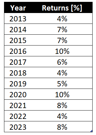
Using this table, let’s go ahead and calculate the different central location metrics.

Mode

The mode is the value that appears most often in a dataset. The following table groups the returns from the hypothetical strategy together and counts their respective occurrences:

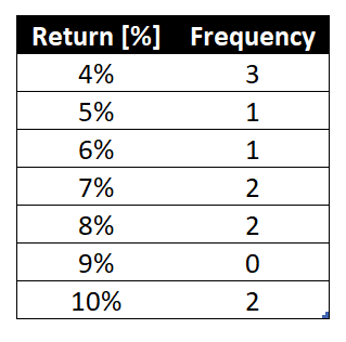
The most frequent value is 4%, with three occurrences. Therefore that is the mode of distribution.

The mode has an advantage over the median and the mean, as the mode can be easily found for both numerical and non-numerical data.

We can also find more than one mode for the same distribution of data. This can limit the ability of the mode to describe the center of the distribution. In some cases, the data set may have no mode at all. It may be better to consider using the median or mean in these cases.

Median

The median is the middle value in a distribution when the values are displayed in ascending or descending order.

Looking at our example (which has 11 observations), the median is 7%. 

4%, 4%, 4%, 5%, 6%, 7%, 7%, 8%, 8%, 10%, 10%

Conveniently, we had 11 values, but let’s consider what happens if we have an even sample size. In the subsequent distribution, we have 12 observations; therefore, the median will be the mean of the two middle values in this case. These are 6 and 7; thus, the median equals 6,5.

2%, 4%, 4%, 4%, 5%, 6%, 7%, 7%, 8%, 8%, 10%, 10%

The median is used when the distribution is not symmetrical because it is less affected by outliers and skewed data.

Mean

The mean, or the arithmetic average, is the sum of the value of each observation in a dataset divided by the number of observations included in that dataset.

E[X] = (1% + 7% + 7% + 10% + 6% + 4% + 5% + 10% + 8% + 4% + 8% ) / 11 = 70%/11 = 6.36%

In our case, we add all the returns and divide this sum by 11, as we have 11 observations, which equals 6,63.

The mean cannot be calculated for non-numerical data, as the values cannot be summed. As it includes every value in the distribution, outliers and skewed distributions influence the mean. In contrast to the mode and the median, the mean can be heavily influenced by outliers (a value that is far apart from most other values).

Measures of Dispersion

Two data sets can have the same mean, but they can be different. Thus to describe data, we need to know the extent of variability. This is given by the measures of dispersion. Measures of dispersion are real and non-negative numbers that help to gauge the spread of data. The measures of dispersion help determine how stretched or squeezed the data is.

Consider the yearly returns of the following two strategies.

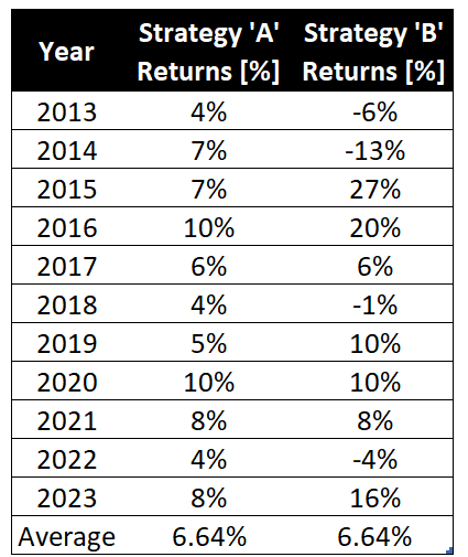
As you can see, both have the same average return, but they certainly have a very different risk profiles: the returns from Strategy ‘A’ are closer to the average, whereas the returns of Strategy ‘B’ are all over the place.

Measures of dispersion are vital as they help to get an understanding of the distribution of data. The value of the measure of dispersion increases along with the diversity of the data. Measures of dispersion are used to describe the variability in data.

Variance

The variance is the average squared deviation from the data set’s mean. This measure looks at the data’s spread about the mean. The variance makes a comparison between the two data sets on the basis of variability. Suppose we have two data sets, A and B, with variances of 3 and 10. This means that data set B is more variable than data set A.

Let’s calculate the variance of returns for Strategy ‘A’:

Variance = (4% - 6.64%)^2 + (7% - 6.64%)^2 + … + (8% - 6.64%)^2 = 0.51%^2

Let’s compare it to the variance of returns of Strategy ‘B’:

Variance = (-6% - 6.64%)^2 + (-13% - 6.64%)^2 + … + (16% - 6.64%)^2 = 1.29%^2

Range

The range is the difference between the dataset’s largest and smallest values. The most important advantage of this measure of dispersion is that it is easy to calculate. On the other hand, it is very sensitive to outliers.

The range of Strategy “A” is 6%, whereas it is 40% in the case of Strategy “B.”

Interquartile Range

The interquartile range is the difference between the first and third quartiles (the 25th and 75th %). The interquartile range takes a look at the middle 50% of observations. If the interquartile range is large, the middle 50% of observations are spaced wide apart.

The main advantage of the interquartile range is that it can be used as a measure of variability if the extreme values are not recorded precisely, as it isn’t affected by the extreme values. In other words, the interquartile range is robust against outliers.

This is also its main disadvantage since it cannot capture the total dispersion of the data appropriately.

In the case of Strategy “A,” the 1st and 3rd Quartilesare 5% and 8%, respectively. As a result, the interquartile range is 3%.

For Strategy “B,” the 1st and 3rd Quartiles are -3% and 13%. Thus, the interquartile range is 16%

Standard Deviation

The Standard deviation (SD) is the most frequently used measure of dispersion and is equal to the square root of the sum of squared deviation from the mean divided by # of observations. In the case of a normal distribution, 68.2% of the datapoints are within 1 standard deviation of the mean.

Let’s take an example from the stock market. XYZ is being traded on the exchange. The traders who want to invest in XYZ will look at its historical return data for the last year. They will assess the extent of scattering of XYZ’s returns over the past year. If the degree of scattering of returns is low, it means less price fluctuation. Thus, the investment will be considered safer. Moreover, if the degree of spread is higher, the price is highly volatile. Therefore, the investment will be considered unsafe in such a case.

In other words, a high dispersion means that the investment will be riskier and vice versa.

Going back to our previously used examples of Strategy “A” and Strategy “B”, we have to take the squared root of the variance we already calculated.

Std. Dev. (Strategy "A") = Sqrt( Variance (Strategy "A") ) = Sqrt(0.51%^2) = 2.25%

Assuming that the returns of Strategy “A” follow a normal distribution (which it does not), 68.2% of the yearly returns will fall within 1 standard deviation of the mean. In other words, within 6.64% ± 2.25%.

In the real world, this would be an outstanding strategy, since it would result in a Sharpe Ratio of 2.95 (not accounting for the risk-free interest rate).

Such high values are only achieved by high-frequency traders and market makers. In the case of retail traders, a Sharpe Ratio over 2 is almost always only achieved by aggressively overfitted backtests.

In the case of Strategy “B,” 68.2% of the returns would fall within 6.64% ± 11.93%. Ignoring the risk-free interest rate, this would be analogous to a Sharpe Ratio of 0.57, which is pretty mediocre by most standards.

Measures of Asymmetry (skewness)

Skewness is a measure of asymmetry that measures the deviation of a variable’s given distribution from the normal distribution, which by definition, is symmetrical on both sides. In intuitive terms, skewness might allow you to identify and take advantage of market mispricings. A distribution can be skewed to the left or the right.

1. Positive Skewness

If the given distribution is shifted to the left and with its tail on the right side, it is a positively skewed distribution or a right-skewed distribution.

As the name suggests, a positively skewed distribution assumes a skewness value greater than zero. If the skewness of a distribution is on the right, that means that the mean value is greater than the median and moves towards the right, and the mode occurs at the highest frequency of the distribution.

2. Negative Skewness

If the given distribution is shifted to the right with its tail on the left side, it is negatively skewed or left-skewed. If a distribution has a negative skew, the skewness value of that distribution is always less than zero. If the skewness of a distribution is on the left, that means that the mean value is less than the median, and the mode occurs at the highest frequency of the distribution.

Investors analyze the skewness while estimating the distribution of returns on investments. If a distribution has a positive skew, investors should expect recurrent small losses and occasionally large returns from investment. A negatively skewed distribution suggests that we`ll have many small wins and a few large losses on our investment.

The financial models that want to estimate an asset’s future performance will consider a normal distribution. However, skewed data can increase the accuracy of a financial model. Stop-losses and take-profits can change the skewness as these orders truncate the distribution eliminating the possibility of extreme values.

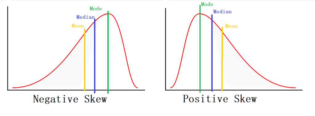
In general, Skewness will impact the relationship of mean, median, and mode for the different kinds of distributions, as presented:

• Symmetrical distribution: Mean = Median = Mode
• Positively skewed distribution: Mode < Median < Mean
• Negatively skewed distribution: Mean < Median < Mode

This can also be intuitively interpreted for trading: Negatively skewed can be misleading since they could be characterized by frequent positive returns (mode) but be negative on average (mean). Consequently, traders might take longer than usual to find out that their strategy is a losing one.

Keep in mind that this generalization is not valid for all possible distributions. If one tail is long and the other is heavy, this may not work.

Most statistics textbooks use the following formula to calculate the skewness of a distribution:

Skew = 3 * (Mean – Median) / Standard Deviation

This formula is known as Person’s Skewness Coefficient. An alternative metric is Fisher’s Measure of Skewness

In the case of Strategy A, the skew is 3 * (6.64% – 7%) / 2.25% = -0.48, meaning that it is a negatively skewed distribution. Thus, although we saw that the Sharpe Ratio was (impossibly) high, larger-than-expected losses could occur.

Measures of Peakedness (Kurtosis)

The fourth moment is called Kurtosis, which measures the so-called “tailedness” of the distribution. Kurtosis can be referred to as the volatility of volatility. It uses the fourth power in the calculation. Therefore, a large value in the tail has more effect on kurtosis than a small value from the middle.

Whereas skewness differentiates extreme values in one versus the other tail, kurtosis measures extreme values on both tails. A distribution with large kurtosis exhibit tail data exceeding the tails of the normal distribution. A distribution with low kurtosis exhibit tail data that are generally less extreme than the tails of the normal distribution.

The normal distribution has a kurtosis of 3. Therefore, we define excess kurtosis (EK) as the difference with respect to 3.

• EK= 0. It has the same tail as a normal distribution, and it’s called Mesokurtic

• EK > 0. It has a fatter tail than a normal distribution, called Leptokurtic. We have more extremely large returns in the tails.

• EK < 0. It has a slimmer tail than the normal distribution, and it’s called Platykurtic. We have fewer extremely large returns in the tails.

Kurtosis is calculated as the ratio between the fourth moment and the squared second moment. This is a mouthful, so let’s break it down:

m4 = sum(Ret - Ret_avg)^4 / n
squared m2 = (sum(Ret - Ret_avg)^2)^2 / n^2

Combining both equations, we construct the formula for Kurtosis:

Kurtosis = m4 / m2^2 =  [sum(Ret - Ret_avg)^4 / n] / (sum(Ret - Ret_avg)^2)^2 / n^2

Finally, Excess Kurtosis is just subtracting 3 from Kurtosis. If you use the KURT() formula in MS Excel, keep in mind that it calculates excess Kurtosis.

In the case of Strategy “A”, the distribution has an Excess Kurtosis of -1.18, meaning that it has thin tails (Platykurtic).

Market returns are mostly leptokurtic due to volatility clustering. A distribution of returns with high kurtosis implies that the investor will experience occasional extreme returns (either positive or negative). This phenomenon is known as kurtosis risk.

The kurtosis risk cannot be explained by variance or SD because higher moments cannot be explained by lower moments. We can find two data sets with the same variance but different kurtosis. Thus, it is important to calculate up to the fourth moment of a distribution of returns.

Frequently Asked Questions

Is a higher standard deviation considered good or bad in trading?

A high standard deviation implies that the data is spread more widely, therefore, is riskier. A low standard deviation implies that the data is closely clustered around the mean and is thus considered a safer investment. Higher dispersion means riskier investment and vice versa.

What type of skewness is better in trading?

A positively skewed distribution should be preferred over a negatively skewed one since the huge gains may cover the frequent but small losses.

Is high kurtosis considered good in trading?

For investors, high kurtosis of the return distribution implies the investor will experience more frequent extreme returns than usual. These returns can be negative or positive, but in any case, the high kurtosis implies larger risks.