When researching trading strategies, walk-forward optimization is, without a doubt, one of the most valuable tools you could incorporate into your workflow. Although the average trader does not even properly backtest their strategies, it is worth considering that most of them lose money on average.

I’ll assume that you already know what walk-forward optimization is about, but you can check out this article I wrote on the topic as a quick refresher on the main aspects and advantages of this technique.

By the end of this article, you’ll be better equipped than most algorithmic traders. So, without any further ado, let’s get started!

Walk-Forward Optimization in Python

I tried to make this article as easily digestible as possible, but the task is by no means easy. This is why I decided to break it down into smaller parts. First, we’ll describe and implement the trading strategy. After having done so, we’ll optimize its parameters. Last but not least, we’ll implement the walk-forward optimization itself.

We will be using Backtesting.py, which is one of the most mature, popular, and reliable backtesting frameworks available for Python. Since it does not have inbuilt capabilities for walk-forward optimization, we will be coding that feature ourselves.

Step 1: Implementing the Trading Strategy in Python

Let’s start by importing the required libraries that we will be using throughout this tutorial and declaring a few parameters. We will first implement the strategy used for doing the walk-forward optimization.

import yfinance as yf
import pandas as pd
from backtesting import Strategy, Backtest
import seaborn as sns
from tqdm import tqdm

TICKER = 'AAPL'
START_DATE = '2015-01-01'
END_DATE = '2022-12-31'
FREQUENCY = '1d'

As you can infer, we’ll use AAPL’s stock price from 2015 to 2022, so let’s fetch the data using yahoo finance!

I removed the timezone awareness of the DateTimeIndex to make things easier down the line.

df_prices = yf_ticker = yf.Ticker(TICKER).history(start=START_DATE,end=END_DATE,interval=FREQUENCY)
df_prices.index = df_prices.index.tz_localize(None)

Our strategy is going the be a simple yet interesting mean-reversion strategy. We will buy the stock whenever the current price is at its lowest. Conversely, we will sell the asset if the price is currently at its highest during the lookback period. We will refer to these prices as high and low watermarks.

Implementing both functions is rather straightforward if we leverage pandas functionalities:

def high_watermark(highs, loockback):
    return pd.Series(highs).rolling(loockback).max()

def low_watermark(mins, loockback):
    return pd.Series(mins).rolling(loockback).min()

Lets us also go ahead and implement the strategy for our backtest:

class BLSHStrategy(Strategy):
    n_high = 30
    n_low = 30

    def init(self):
        self.high_watermark = self.I(high_watermark, self.data.Close, self.n_high)
        self.low_watermark = self.I(low_watermark, self.data.Close, self.n_low)

    def next(self):
        if not self.position:
            if self.low_watermark[-1] == self.data.Close[-1]:
                self.buy()

        elif self.high_watermark[-1]  == self.data.Close[-1]:
            self.position.close()

The code is pretty straightforward, but let’s go through it step by step:

• During initialization, we create two indicators: high_watermark and low_watermark. Both lookback periods are defined in n_high and n_low and are by no means required to be equal.
• The next method is where the magic happens. If we don’t already hold a position in AAPL, we check if the price is currently at the 30-day lowest. If so, we will issue a buy order. On the other hand, if we already hold a position and the price is at its highest, we will issue an order to close the position.

To keep things simple, we will assume commission-free trading. By only selling if we hold a position, we force our strategy to be long-only.

bt = Backtest(df_prices, BLSHStrategy, cash=10_000, commission=0,exclusive_orders=True)
stats = bt.run()
stats

Step 2: Optimizing the parameters of the strategy

The next step is optimizing the high and low watermark lookback period parameters. For this, we will use the Backtesting library’s optimize() method. This method will run the backtest for all the combinations of the parameters passed to it.

bt = Backtest(df_prices, BLSHStrategy, cash=10_000, commission=0,exclusive_orders=True)

stats, heatmap = bt.optimize(
    n_high=range(20, 60, 5),
    n_low=range(20, 60, 5),
    # constraint=lambda p: p.n_high > p.n_low,
    maximize='Equity Final [$]',
    method = 'grid',
    max_tries=56,
    random_state=0,
    return_heatmap=True)

Let’s take a few seconds and take a closer look at the most relevant parameters:

• We test different combinations of the parameters n_high and n_low. We will try values between 20 and 60. To reduce processing times, we will only test multiples of 5.
• As with any optimization, we must choose a target variable to maximize (or minimize). In this case, we will maximize the profitability of the strategy. Keep in mind that this variable completely ignores the incurred risk. This could be accounted for by maximizing the Sharpe Ratio instead.
• We can also add constraints. We won’t introduce any in this case, but I left the feature commented out in case you want to use it.

The method returns two variables: the statistics of the best-performing combination and a matrix with the results of all the combinations we tested. We already know what the stats output looks like, so let’s jump right into the heatmap!

sns.heatmap(heatmap.unstack())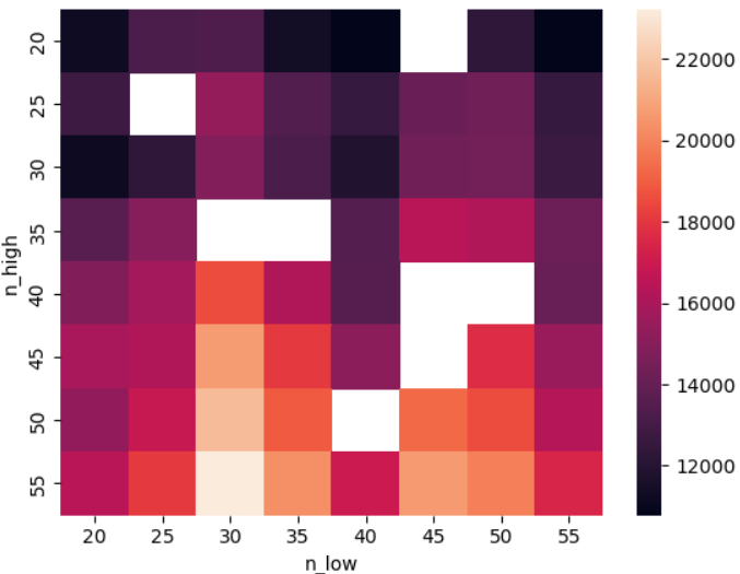

As a side note, it’s worth mentioning that the empty cells are there because we limited the number of tries to 56.

Step 3: Walk-Forward Optimization of the Strategy

Backtesting.py has no inbuilt functionalities for performing walk-forward optimization, but we can extend the library to perform this task with a few tweaks!

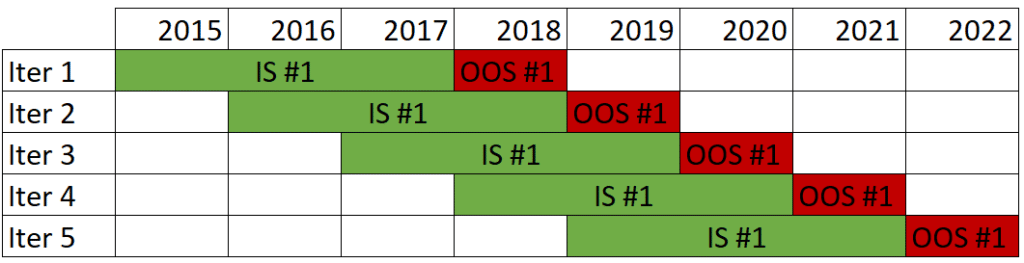
Having 8 years of data, we will do 5 iterations. Each iteration will use 4 years of data, where the first 3 will be used for optimizing the parameters (in-sample data) and the fourth year as a test set (out-of-sample data).

from datetime import datetime
iterations = [
    {
        'in_sample': [datetime(2015,1,1),datetime(2017,12,31)],
        'out_of_sample': [datetime(2018,1,1),datetime(2018,12,31)]
    },
    {
        'in_sample': [datetime(2016,1,1),datetime(2018,12,31)],
        'out_of_sample': [datetime(2019,1,1),datetime(2019,12,31)]
    },
    {
        'in_sample': [datetime(2017,1,1),datetime(2019,12,31)],
        'out_of_sample': [datetime(2020,1,1),datetime(2020,12,31)]
    },
    {
        'in_sample': [datetime(2018,1,1),datetime(2020,12,31)],
        'out_of_sample': [datetime(2021,1,1),datetime(2021,12,31)]
    },
    {
        'in_sample': [datetime(2019,1,1),datetime(2021,12,31)],
        'out_of_sample': [datetime(2022,1,1),datetime(2022,12,31)]
    },    
]

The following script is where all the meat is! We are putting everything together to perform the walk-forward optimization I promised!

The code is a little messy/daunting, so let me break it into smaller chunks!

1. Iterate over the list of dictionaries, each containing the in-sample and out-of-sample periods.
2. Filter the data only to include the relevant dates.
3. Calculate the optimal parameters using the in-sample data.
4. Run the backtest for the out-of-sample data using the optimal parameters.
5. Append relevant metrics to a list of results.

report = []
# 1: We iterate over the list of dictionaries
for iter in tqdm(iterations):
    # 2: We filter the data to only include the relevant dates.
    df_is = df_prices[(df_prices.index >= iter['in_sample'][0]) & (df_prices.index <= iter['in_sample'][1])]
    df_oos = df_prices[(df_prices.index >= iter['out_of_sample'][0]) & (df_prices.index <= iter['out_of_sample'][1])]

    #3: Calcualte the optimal parameters using the in-sample data. 
    bt_is = Backtest(df_is, BLSHStrategy, cash=10_000, commission=0,exclusive_orders=True)
    stats_is, heatmap = bt.optimize(
        n_high=range(20, 60, 5),
        n_low=range(20, 60, 5),
        maximize='Equity Final [$]',
        method = 'grid',
        max_tries=64,
        random_state=0,
        return_heatmap=True)
    # 4: Run the backtest for the out-of-sample data using the optimal parameters.
    BLSHStrategy.n_high = stats_is._strategy.n_high
    BLSHStrategy.n_low = stats_is._strategy.n_low
    bt_oos = Backtest(df_oos, BLSHStrategy, cash=10_000, commission=0,exclusive_orders=True)
    stats_oos = bt_oos.run()
    
    # 5: Append relevant metrics to a list of results
    report.append({
        'start_date': stats_oos['Start'],
        'end_date': stats_oos['End'],
        'return_strat': stats_oos['Return [%]'],
        'max_drawdown':stats_oos['Max. Drawdown [%]'],
        'ret_strat_ann': stats_oos['Return (Ann.) [%]'],
        'volatility_strat_ann': stats_oos['Volatility (Ann.) [%]'],
        'sharpe_ratio': stats_oos['Sharpe Ratio'],
        'return_bh': stats_oos['Buy & Hold Return [%]'],
        'n_high': stats_oos._strategy.n_high,
        'n_low': stats_oos._strategy.n_low
    })

Here’s a Pandas DataFramewith the results:

pd.DataFrame(report)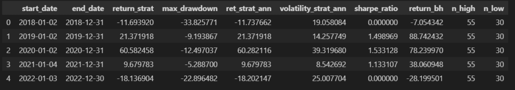

Step 4: Further Improvements

By now, we already have a walk-forward optimization function that works. However, there are a few things that we can improve, and I conveniently ignored them in the previous section to make them stand out more.

• Add Exposure Percentage: To compare apples to apples, it is important to know the exposure percentage of the strategy. A strategy with the same returns as the buy and hold that only holds the asset 50% of the time is considered better because it is less exposed to the market.
• Scale the Buy & Hold Returns: To compare the strategy to its benchmark, we will scale the returns of the Buy & Hold to match the exposure of our strategy.
• Add in-sample Returns: it is worthwhile to compare the returns of the in-sample and out-of-sample periods. If the OOS backtests yield much lower returns, we can conclude, with a high degree of certainty, that we are overfitting.
• Plot the heatmaps of each optimization: Although not strictly a requirement, it is desirable for the 5 heatmaps to be somewhat similar.

from tqdm import tqdm
report = []
for iter in tqdm(iterations):
    df_is = df_prices[(df_prices.index >= iter['in_sample'][0]) & (df_prices.index <= iter['in_sample'][1])]
    df_oos = df_prices[(df_prices.index >= iter['out_of_sample'][0]) & (df_prices.index <= iter['out_of_sample'][1])]

    bt_is = Backtest(df_is, BLSHStrategy, cash=10_000, commission=0,exclusive_orders=True)
    stats_is, heatmap = bt_is.optimize(
        n_high=range(15, 40, 5),
        n_low=range(15, 40, 5),
        maximize='Equity Final [$]',
        method = 'grid',
        max_tries=64,
        random_state=0,
        return_heatmap=True)
    BLSHStrategy.n_high = stats_is._strategy.n_high
    BLSHStrategy.n_low = stats_is._strategy.n_low
    bt_oos = Backtest(df_oos, BLSHStrategy, cash=10_000, commission=0,exclusive_orders=True)
    stats_oos = bt_oos.run()
    report.append({
        'start_date': stats_oos['Start'],
        'end_date': stats_oos['End'],
        'return_strat': stats_oos['Return [%]'],
        'max_drawdown':stats_oos['Max. Drawdown [%]'],
        'ret_strat_ann': stats_oos['Return (Ann.) [%]'],
        'volatility_strat_ann': stats_oos['Volatility (Ann.) [%]'],
        'sharpe_ratio': stats_oos['Sharpe Ratio'],
        'return_bh': stats_oos['Buy & Hold Return [%]'],
        'n_high': stats_oos._strategy.n_high,
        'n_low': stats_oos._strategy.n_low,
        'exposure': stats_oos['Exposure Time [%]'],
        'bh_scaled': stats_oos['Buy & Hold Return [%]'] * stats_oos['Exposure Time [%]'] / 100,
        'is_heatmap': heatmap,
        'sharpe_is': stats_is['Sharpe Ratio'],
    })

Finally, let’s plot the heatmap of each optimization:

import matplotlib.pyplot as plt
import math
plt.rcParams['figure.figsize'] = [20, 10]

rows = len(report)
for idx, res in enumerate(report):
    plt.subplot(math.floor(rows/2), math.ceil(rows/2), idx+1)
    plt.title(f"Iter # {idx+1} - Year {res['start_date'].year}")
    sns.heatmap(res['is_heatmap'].unstack())
plt.show()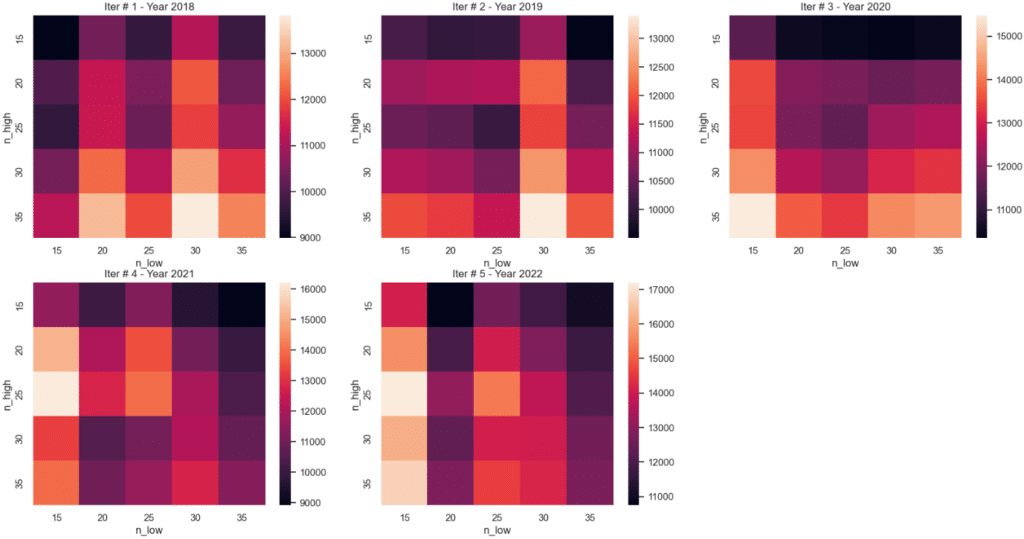

Conclusion

As you can see, implementing this feature is not rocket science but is definitely out of reach for the average algorithmic trader. I hope to have conveyed the advantages of incorporating this technique int your workflow, and please don’t hesitate to drop a comment if you have any further questions!