When measuring the performance of a trading strategy, the Sharpe Ratio stands out as the most widely used metric. This is because it is a straightforward and easy-to-understand risk-adjust return metric.

Although the formula is easy to understand, calculating each component is an error-prone task.

This is why in this article, I will show you how to calculate the Sharpe Ratio in a step-by-step fashion using only Microsft Excel.

So, without any further ado, let’s get started.

Sharpe Ratio in Excel

In order to keep things organized, I will break down the formula into its components and cover each individually before putting everything together.

Just as a reminder, the formula of the Sharpe Ratio (SR) is as follows:

SR = (E[Return] – rfr) / Std[Return]

Where:

• E[Return]: the expected return of the asset. Historical data is used to calculate it, and it is oftentimes expressed in yearly terms.
• Rfr: the risk-free rate of return. It is the yearly interest that investors can achieve by purchasing T-Bills.
• Std[Returns]: The standard deviation of the returns. It is a statistical measure of dispersion used to represent an asset’s risk.

Getting Historical Stock Prices in Excel

As you might have already noticed, we require at least a year of daily prices before calculating each component. Luckily for us, we can use the “STOCKHISTORY “function that is included in Excel!

In this example, we will calculate the Sharpe Ratio of the SPY, an ETF designed to track the S&P 500 stock market index. The following animation shows how to use the “STOCKHISTORY “function.

In case you want to copy the formula, here it is:

=STOCKHISTORY("SPY",TODAY()-365,TODAY(),0,1,0,1)

Calculating the Yearly Return of an Asset in Excel

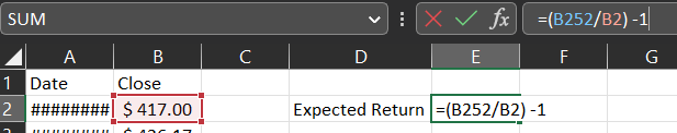
Given the fact that we have exactly one year’s worth of data, we can go ahead and calculate the yearly return by just using the most recent price and dividing it by the first one (and subtracting 1).

Calculating the Yearly Volatility of an Asset in Excel

Calculating the yearly volatility of the asset is not as straightforward as the yearly return. The standard deviation is the squared root of the sum of the squared excess returns divided by the sample size. This is a mouthful and is best understood in mathematical terms:

s = sqrt [Σ(Ri – R)^2 / (n)]

• Ri: the return of the asset on day “i”
• R: the average daily return of the asset over the entire period.

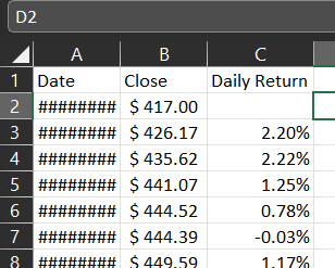
Let’s start by calculating the daily returns. In cell C3, write the following formula:

=(B3/B2)-1

Copy that formula and paste it into the remaining rows. It is also nice to format it as a percentage. The top of your table should now look similar to what I’ve got here:

We now need the average daily return, which I’m showing howe to calculate in the following animation:

In column “D,”we will calculate the section of the formula that is bold: sqrt [Σ(Ri – R)^2 / n]. As usual, here’s an animation showing how to do it:

Make sure to use the “$” sign on the average daily return so that the cell remains fixed when pasting it for the remaining cells of column “D“. The formula is as follows:

=(C3-$G$3)^2

On cell “G4“, calculate the sum of column “D“:

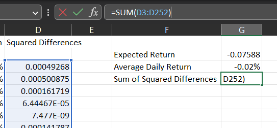
We’re almost there! If you look again at the formula, we now have to divide it by the sample size and take the square root. Let’s do that in cell “G6“:

=SQRT(G4/COUNT(D3:D252))

We now arrived at the daily standard deviation. If you paid close attention, you might remember that we need the yearly volatility, so we need to multiply it by the square root of 252. Why 252? Because that is commonly used as the number of trading days within a year!

=G6*SQRT(252)

Now that you’ve gone through the hassle of calculating this metric manually, I can show you how to do it more efficiently:

=STDEV.P(C3:C252) * SQRT(252)

Don’t get mad at me! I really think there is pedagogical value in having calculated it manually.

Last Step: Calculating the Sharpe Ratio in Excel

We already have the yearly return and risk! The only component missing is the risk-free rate, which we can get from multiple sources (here’s the link to MarketWatch). I’m using the 12-month T-Bill, which is a reasonable assumption considering that we are doing everything in yearly terms. As of writing this article, the rate is 4.51%.

It is worth mentioning that traders tend to ignore the risk-free rate and instead calculate the Sharpe Ratio by just dividing the yearly return by the volatility. This is a reasonable simplification in cases where we are comparing two strategies or assets over the same period. For completeness, I will be using the risk-free rate for my calculations:

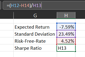
Since I’m writing this article on March 2023, the Sharpe Ratio is negative (-0.52).

Frequently Asked Questions

What is a good Sharpe Ratio?

Retail investors oftentimes say that a Sharpe Ratio below one is poor, whereas a value above one is considered good. Despite the convenience of having such simple rules, this claim is misleading.

Sharpe Ratios should be used to compare different alternatives. A single Sharpe Ratio without any context or reference is relatively useless.

If you had just bought the SPY on May 2020 and held it for a year, you would have achieved a Sharpe Ratio of 2.77. It could be argued that an active strategy that yielded a Sharpe Ratio of 1.01 during the same period performed poorly. Conversely, a strategy with a Sharpe Ratio of 1.01 during 2022 would be considered excellent.

Market-makers and high-frequency trading firms can achieve Sharpe Ratio greater than two over prolonged periods. Other than that, it is a good rule of thumb to discredit any trader with a backtest promising such a performance. He is either ignorant or a Nigerian prince.